 2019, Vol. 50
中国海洋湖沼学会主办。
文章信息
- 李国庆, 高艳秋, 张继才. 2019.
- LI Guo-Qing, GAO Yan-Qiu, ZHANG Ji-Cai. 2019.
- Ekman模型时间变化风应力系数的伴随参数估计
- ADJOINT PARAMETER ESTIMATION OF TIME-VARYING WIND DRAG COEFFICIENT FOR AN EKMAN MODEL
- 海洋与湖沼, 50(5): 979-993
- Oceanologia et Limnologia Sinica, 50(5): 979-993.
- http://dx.doi.org/10.11693/hyhz20190100029
文章历史
-
收稿日期:2019-01-29
收修改稿日期:2019-04-19


2. 自然资源部第二海洋研究所 卫星海洋环境动力学国家重点实验室 杭州 310012
2. State Key Laboratory of Satellite Ocean Environment Dynamics, Second Institute of Oceanography, Ministry of Natural Resources, Hangzhou 310012, China
风是驱动海洋环流的重要因素, 与之相关的风应力则是计算海气界面动量交换的基本指标。风应力拖曳系数(Wind Stress Drag Coefficient, WSDC)是计算风应力的关键参数, 因此风应力系数对于与海面风相关的上层海洋过程具有很大的影响(Peng et al, 2015)。在前人的研究中, 风应力系数常被假设为常数(Konishi et al, 1985; Jones et al, 1998), 或被设置为风速的线性函数(Garratt, 1977; Wu, 1980, 1982), 或被设为风速的非线性函数(Large et al, 1981; Powell et al, 2003; Large et al, 2009; Zijlema et al, 2012; Edson et al, 2013; Peng et al, 2015), 具体关系如图 1所示。目前, 风应力系数随风速非线性变化, 尤其是在高风速条件下, 已被广泛接受与认可(Powell et al, 2003; Hwang, 2005; Jarosz et al, 2007; Maurer et al, 2015)。由于涉及到海气相互作用过程, 风应力系数的确定是海洋科学和大气科学领域的一个难点问题, 其困难根源来自于湍流问题。湍流在时间和空间尺度的多变性, 导致求解湍流问题异常困难。近惯性频率段的海洋观测表明, 与板状模型相比, 湍流封闭模型能更好地预测风生流(Weller et al, 1996)。目前的湍封闭模型存在多种选择, 例如依赖于Richardson数的模型、k-ε模型、M-Y模型、Prandtl混合长度模型、KPP模型等, 它们在不同的区域、不同的事件中, 都发挥了重要的作用(Pacanowski et al, 1981; Ferreira et al, 2004; Mellor, 2004; Wang et al, 2010)。但是, 由于海洋环境往往会随空间和时间发生变化, 再加上观测数据的不足, 各个湍流模型的普适性受到限制, 具体表现为不同模型计算出的参数差别较大, 没有哪种模型能精准适用于所有海域。
 |
| 图 1 前人公式中风应力系数与风速的关系 Fig. 1 Wind Stress Drag Coefficients (WSDCs) as a function of wind speed from previous works |
伴随同化方法是在严格的数学理论基础上发展起来的(Thacker et al, 1988)。伴随同化将变分原理与最优控制理论相结合, 流体力学方程组及其初、边值条件作为约束条件, 使得依据具体问题设计的代价函数达到最小(Sasaki, 1970)。近几十年以来, 对于未知参数的确定, 数据同化方法发挥了重要作用, 以伴随同化方法和卡曼滤波(Kalman Filter)同化参数估计为代表(Kalman, 1960; Daley, 1991; Evensen, 1992; Fisher et al, 1995; Evensen et al, 1996; Navon, 1997)。同化参数估计的思路在于, 由于动力过程的复杂性和参数的未知性, 海洋模型所反应的动力系统类似于“黑箱子”, 但是“黑箱子”的输出却是可以观测的, 即海洋观测资料; 这就提供了一种可能性, 基于数学物理反问题的思路, 我们可以从输出(观测资料)去反推输入的控制变量(参数)。近年来同化参数估计在许多实际问题中得到应用(Yu et al, 1991; Das et al, 1992; Ullman et al, 1998; Heemink et al, 2002; Lv et al, 2004; Wakelin et al, 2009; Zhang et al, 2009; Kim et al, 2015; Zhang et al, 2015; Gharamti et al, 2017)。Yu等(1991)验证了Ekman伴随同化模型优化风应力系数和海水涡动黏性系数剖面的能力。Yu等(1992)探究了初始条件对反演结果的影响, 一定程度上优化了Ekman模型的初始流速。Zhang等(2009)分析了伴随同化方法反演改进的Ekman模型中风应力系数的部分敏感性, 包括:优化算法、调整参数的步长、伴随方程的反积分时间和正则化参数, 但是未涉及到实际海洋数据。本文采用一个改进的Ekman模型, 基于时间分布参数的假设, 建立相关算法, 利用伴随同化方法反演了随时间变化的风应力系数, 并运用孪生实验和实际实验对该方法进行了验证; 数值实验结果表明, 该方法对利用风速和上层流速的观测值反演时间分布的风应力系数是有效的, 有利于提高风应力系数的取值合理性和模拟准确度。
本文结构如下:第一节简要描述了改进的Ekman模型、伴随同化方法以及数值实验运算过程; 第二节进行了一系列孪生实验, 对随时间变化的风应力拖曳系数反演问题进行了敏感性分析实验; 第三节利用百慕大锚系实验平台风速和流速数据, 反演该区域随时间变化的风应力拖曳系数, 并通过比较模拟和观测流速, 验证了该方法的有效性; 第四节是讨论和总结。
1 模型描述 1.1 控制方程本文采用修正的Ekman模型(Yu et al, 1991), 其控制方程为:
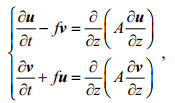 (1)
(1)其中, t为时间, z为水深, 取z轴垂直向上为正, 且在海洋表面处z=0, u(向东为正向)和v(向北为正向)为海洋各深度处水平方向的流速分量, f为Coriolis参数, A为涡动黏性系数。对于方程(1), 初始条件的设置与吕咸青(2001)相同。
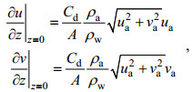
相应的边界条件为:
 (2)
(2) (3)
(3)其中, Cd为风应力拖曳系数, ρa和ρw分别为空气和海水的密度, ua(向东为正向)和va(向北为正向)为10m高空处风速的水平分量, H0为Ekman层的深度。
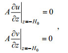
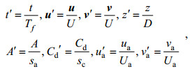
由于上述参数的物理性质不同, 具有不同的单位(Gill et al, 1981; Luenberger et al, 1984)。在方程中引入无量纲变量(Yu et al, 1991):
 (4)
(4)其中,
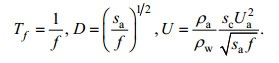 (5)
(5)其中, t'、u'、v'、z'、A'、Cd'、ua'、va'是原变量的无量纲变量, Tf、U、D、sa、sc、Ua是公式(4)中对应变量的变换系数, 其他变量的定义与公式(2)相同。
得到方程:
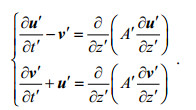 (6)
(6)因下文中这8个变量都是使用带撇的无量纲变量, 为了书写方便和容易理解, 省略这些变量的撇号。
1.2 伴随方程构造代价函数:
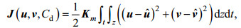 (7)
(7)其中, 

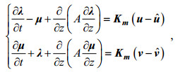 (8)
(8)其中, λ和μ分别是u和v的拉格朗日乘子(又称为伴随变量)。边界条件和初始条件的设置与吕咸青(2001)相同。
代价函数J关于风应力拖曳系数的梯度计算方法为:
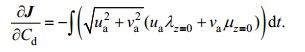 (9)
(9)由此可得:
(1) 风应力拖曳系数的时间分布反演
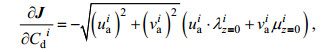 (10)
(10)(2) 风应力拖曳系数的恒定值反演
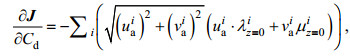 (11)
(11)其中, i是时间指标。
1.3 差分格式及数值实验过程本文采用的有限差分格式是Crank-Nicholson格式(O’Brien, 1986)。控制方程(4)的差分形式为:
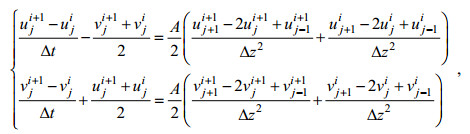 (12)
(12)其中, Δt和Δz分别代表时间和垂向步长。
伴随方程(6)的差分形式为:
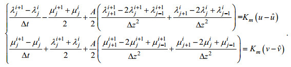 (13)
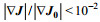
(13)数值实验的运算过程为: 1)估计控制参数A的合理输入值, 和Cd的合理初始值; 2)利用控制方程(6)积分, 得到u和v的模拟值; 3)模拟值与观测值的差驱动伴随方程(8)反向积分, 得到λ和μ的值; 4)利用方程(9)计算代价函数关于Cd的梯度
实际实验和理想实验的运算过程不同之处在于, 1)理想实验的u和v观测值是通过本文模型模拟得到的, 而实际实验采用的是实测数据; 2)理想实验的风场是由数学函数生成的, 而实际实验的是实测风场数据。
2 理想实验理想实验的模型参数设置如下:
T=10d(总积分时间), Δt=0.5h;
H0=100m, Δz=5m;
u0=0, v0=0(冷启动, 即海流初始时刻处于静止状态);
f=10-4s-1;
A=0.8×10⁻² m2/s;
ρa=1.2kg/m3, ρw=1.025×10³kg/m3;
sa=5.0×10⁻² m2/s, sc=1.2×10⁻³, Ua=10m/s。
2.1 不同风速时间分布下风应力拖曳系数的反演正如引言中提到的, 风应力拖曳系数和风速都是和时间有关的变量; 另外, 真实海洋中风速随时间的变化是复杂的, 而风应力拖曳系数随时间变化的具体分布亦是未知的。因此, 有必要尝试不同时间变化风速分布下风应力拖曳系数的反演。结合一次函数、二次函数和三角函数, 共进行了6组实验, 风应力拖曳系数的初始值全部设为1.2×10⁻³。
方案1, Cd(i)=0.0012+0.00096cos(2πiΔt/10);
方案2, Cd(i)=-0.00006×(iΔt/24-5)2+0.0024;
方案3, Cd(i)=0.00006×(iΔt/24-5)2+0.00072;
方案4, Cd(i)=(4.32+iΔt/24)/6000;
方案5, Cd(i)=(14.4-iΔt/24)/6000;
方案6, Cd(i)=0.00144;
其中, i是时间步, i=0—T/Δt。
每组风速的分布有6种策略:
策略1: ua(i)=10cos(2πiΔt/10)+50 m/s, va(i)=0;
策略2:ua(i)=-0.8(iΔt/24-5)2+40 m/s, va(i)=0;
策略3: ua(i)=0.8(iΔt/24-5)2+20 m/s, va(i)=0;
策略4: ua(i)=0.0205i+11 m/s, va(i)=0;
策略5: ua(i)=-0.0205i+31 m/s, va(i)=0;
策略6: ua(i)=8 m/s, va(i)=0。
6组风应力拖曳系数给定值和反演值如图 2a—图 2f所示, 代价函数下降情况如图 2g—图 2l所示; 第1—6组同化前后风应力拖曳系数的均方根误差见图 3。其中, 代价函数反映了模拟结果和观测流速的“距离”, 均方根误差RMSE则反映了同化前后风应力拖曳系数的绝对误差。从图 2g—图 2l可见, 经过600次迭代后, 6组实验的代价函数均显著下降, 结果表明:在6种风速分布条件下反演给定的6组风应力拖曳系数分布均获得成功, 给定值和反演值具有良好的一致性。同时, 同化后代价函数下降了2—3个数量级, 均方根误差下降了1—2个数量级, 且第4种风速策略在各组中下降最为明显。综上所述, 6组风应力拖曳系数分布在6种风速分布下均能成功反演, 其中在风速策略4下反演效果最好。
 |
| 图 2 第1—6组风应力拖曳系数给定值与反演值(a—f)以及约化的代价函数log(J/J0)(g—l) Fig. 2 Prescribed and inverted WSDCs (a—f) and log(J/J0) (g—l) in Group 1—Group 6 |
 |
| 图 3 第1—10组实验中约化的均方根误差log(RMSE/RMSE0) Fig. 3 log(RMSE/RMSE0) in Group 1—Group 10 |
为了提高同化效率, 参数的初始猜测应尽可能合理(Zhang et al, 2008)。因此, 本节设置了第7组实验, 探讨不同风应力拖曳系数初始猜测对反演结果的影响, 根据Leredde等(1999), Zhang等(2008), Kirincich等(2009), Yoshikawa等(2010), 将方案7-1—方案7-5的风应力拖曳系数初始猜测值分别设为0.00018、0.00072、0.0012、0.0022和0.003。给定的风应力拖曳系数分布选取为2.1节第一组的分布, 基于2.1节中对反演结果的分析和图 1风应力系数随风速的变化情况, 将风速分布设定为分段函数(图 4a), 目的是体现风速常数分布、由小变大和由大变小的过程:
 |
| 图 4 第7组实验中风速随时间的分布(a)、风应力拖曳系数给定值与反演值(b)以及log(J/J0)(c) Fig. 4 Wind speed as a function of time (a), prescribed and inverted WSDCs (b) as well as log(J/J0) (c) in Group 7 |
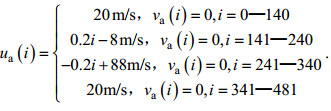 (14)
(14)第7组风应力拖曳系数给定值和反演值如图 4b所示, 代价函数下降情况如图 4c所示, 同化前后的代价函数和均方根误差见图 3。图 4c显示, 经过1600次迭代后, 方案7-1—方案7-5的代价函数均显著下降。从图 4b可以看出, 除了开头和结尾部分, 其余时间段, 方案7-1—方案7-5都成功反演出风应力拖曳系数给定值; 在开头和结尾部分, 方案7-1—方案7-4反演出的风应力拖曳系数低于给定值的程度依次降低, 方案7-5则高于给定值, 且程度大于方案7-4。图 3显示同化后, 代价函数均下降了3个数量级, 均方根误差均下降了1—3个数量级, 在方案7-1—方案7-4中方案7-4下降最明显。实验表明, 与风应力拖曳系数给定值的初始值最接近的初始猜测值反演结果最好。所以基于本组的分析, 以下的理想实验均采用本组给定的风应力拖曳系数分布、风速分布和风应力拖曳系数初始猜测值0.0022。
2.3 独立风应力拖曳系数个数的影响Das等(1991)认为独立变量的个数应该跟观测数据的数量有关, 两者之比不能过大。Ullman等(1998)认为由于观测资料数量的限制, 不可能把每一个网格的系数都作为独立变量; Heemink等(2002)认为太多的独立变量会给参数识别带来困难, 应该根据参数梯度的空间分布确定独立变量的数量及其位置。本节设置了第8组实验, 探讨模拟结果对独立风应力拖曳系数个数的敏感性, 实现方法为在计算时间段内, 按照某设定的间隔均匀选取一些点作为独立的风应力拖曳系数, 其余时间点的风应力拖曳系数由这些独立的风应力拖曳系数线性插值得到。方案7-4和方案8-1—方案8-5分别取独立点个数为480、160、120、96、60和30, 对应的间隔分别为0.5h、1.5h、2.0h、2.5h、4.0h和8.0h。
本组代价函数下降情况如图 5g所示, 方案7-4、方案8-1、方案8-2、方案8-3、方案8-4和方案8-5的风应力拖曳系数给定值和反演值如图 5a—图 5f所示, 同化前后的代价函数和均方根误差见图 3。从图 5可以看出, 方案7-4、方案8-1和方案8-3成功反演了给定的风应力拖曳系数。图 5g显示, 方案7-4和方案8-1—方案8-5的代价函数均发生显著下降。图 3反映出, 同化后, 代价函数下降了3—4个数量级, 均方根误差下降了2—3个数量级, 其中方案8-3下降的最显著。综上所述, 当独立风应力拖曳系数个数取为96时, 能反演出令人满意的结果。独立变量数量的选取会显著影响反演结果, 根据实际情况合理确定, 有利于加快同化效率以及减少观测数据误差。
 |
| 图 5 第8组实验的风应力拖曳系数给定值与反演值(a—f)以及log(J/J0)(g) Fig. 5 The prescribed and inverted WSDCs (a—f) and log(J/J0)(g) in Group 8 注: a—f分别为独立点数为480、160、120、96、60和30的情况 |
真实的流速和风速观测数据是有误差的, Zhang等(2008)认为误差增加到一定范围, 反演结果的失真度会随之增加。本节设置了第9组实验, 探讨误差对反演风应力拖曳系数的影响, 处理方法为将观测值u(i, j), v(i, j)和ua(i)分别用(1+pri)u(i, j), (1+pri)v(i, j)和(1+pri)ua(i)代替, 其中ri为介于(-1, 1)的随机误差, p值决定了最大误差的值。方案8-3和方案9-1—方案9-5分别取最大误差为0%、3%、6%、10%、13%和20%。
本组风应力拖曳系数给定值和反演值如图 6a所示, 代价函数下降情况如图 6b所示, 同化前后的代价函数和均方根误差见图 3。图 6b显示, 本组所有方案的代价函数均发生显著下降。图 6a显示, 方案8-3、方案9-1和方案9-2成功反演出风应力拖曳系数; 方案9-3、方案9-4和方案9-5的反演结果在某些时刻点有所失真, 但依然能反演出风应力拖曳系数的整体趋势。图 3显示, 同化后, 代价函数均下降了2—3个数量级, 均方根误差均下降了2—3个数量级, 随着最大误差依次增加, 代价函数和均方根误差下降数量级依次减小。所以, 考虑风速和流速观测数据误差, 本文的伴随同化模型依然能有效地反演出风应力拖曳系数, 随着观测误差的增加, 反演效果依次变差。
 |
| 图 6 第9、10组实验的风应力拖曳系数给定值与反演值(a、c)和log(J/J0)(b、d) Fig. 6 Prescribed and inverted WSDCs (a, c) and log(J/J0) (b, d) in Group 9 and Group 10 |
真实海洋中, 观测资料在空间上是不连续的或者可能部分缺失, 因此本组尝试使用部分深度的数据进行反演, 设置了第10组实验, 探讨不同深度的数据缺失对风应力拖曳系数反演的影响, 包括方案8-3、方案10-1、方案10-2、方案10-3和方案10-4, 分别对应使用0—20层、0—10层、0—5层、0—2层以及10—20层流速数据的情况。
本组风应力拖曳系数给定值和反演值如图 6c所示, 代价函数下降情况如图 6d所示, 同化前后的代价函数和均方根误差见图 3。图 6d显示, 方案8-3、方案10-1、方案10-2和方案10-3的代价函数均发生显著下降, 使用的数据层位越少, 代价函数收敛速度越快。图 6c显示, 方案8-3、方案10-1和方案10-2均成功反演出风应力拖曳系数, 反演结果依次变差; 方案10-3能反演出风应力拖曳系数的整体趋势, 但有一定程度失真。从图 3看出, 同化后, 方案10-4反演失败, 其余方案的代价函数下降了1—3个数量级, 均方根误差下降了1—3个数量级, 随着使用数据层位的减少, 两者下降的程度依次降低。从上述分析得出, 风应力拖曳系数的反演对上层观测数据更加敏感, 使用的上层观测深度越深, 反演结果越成功, 这是因为Ekman流是由风力驱动的海洋上层水形成的, 对上层观测数据的敏感性最大。
3 实际实验及结果分析 3.1 数据分析与处理本文所使用的风速和流速观测数据来自百慕大锚系试验平台(Bermuda Testbed Mooring, BTM)第23次观测的数据(如图 7所示)。BTM位于百慕大东南80km(31°44′N, 64°10′W)处, 该设备于1994年6月首次部署, 旨在开发测试传感器、分析仪和辐射计等新仪器, 进行高频率、长期、跨学科的数据收集, 为卫星遥感传感器提供标定和验证数据, 以及可以捕获恶劣天气和高海况期间连续的数据等(Dickey et al, 1998; Zedler et al, 2002; Jiang et al, 2007; Black et al, 2008)。
 |
| 图 7 研究区域、百慕大锚系试验平台(Bermuda Testbed Mooring, BTM)位置(a)以及观测仪器图(b) Fig. 7 The study area and Bermuda Testbed Mooring (BTM) position (a) and observation instruments diagram (b) |
本文选取了2005年12月21日0点—2005年12月31日0点, 共10d的数据。风速数据U由海表面浮标塔上的风速计进行测量, 时间分辨率为5min。根据Dickey(2001)和Black等(2008), 风速计位于海面上方4.4m处, 利用Large等(1995)提出的公式和Zedler(1999)概述的方法计算出海表面上方10m处的风速估计值U10。U和U10时间序列如图 8a所示, 该时段有两个较大的风速峰值, 分别在12月24日和12月27日附近, 整体风速的分布包括平缓、升高、降低等完整的风速变化过程, 该时段的U10最大值和平均值分别为17.66m/s和7.57m/s。流速数据由海面下200m深处的声学多普勒流速剖面仪(Acoustic Doppler Current Profiler, ADCP)进行测量, 时间分辨率为15min, 垂向分辨率为3m, 采样深度为23.69—188.69m, 图 8b—图 8d分别展示了23.69、50.69和74.69m深度的流速时间序列。
 |
| 图 8 原始风速U和风速U10的时间序列(a)以及2005年12月21—31日观测到的23.69、50.69和74.69 m处流速向东的分量u和向北的分量v的时间序列(b—d) Fig. 8 The time series of the original wind speed U and wind speed U10 (a) and the time series of eastward and northward current components u and v for 23.69 m, 50.69 m, and 74.69 m, respectively (b—d) |
总流速Utotal(t)包含近惯性流速Uni(t)和潮流流速Utidal(t), Uni(t)又由风生流速Uek(t)和地转流速Ugeo(t)两部分构成(公式(14), Chereskin, 1995; Chereskin et al, 2009; Roach et al, 2015; Liu et al, 2018):
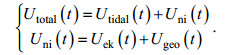 (15)
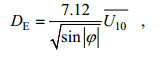
(15)本文主要分析风生流速Uek(t), 需要把其余两个流速成分滤除。Utidal(t)可以利用Zhang等(2009)提及的希尔伯特变换(Hilbert transform)带通滤波方法去掉, 图 9a展示了时间序列流速的频谱分析, 根据分析结果将带通频段取为[0.96 1.2]f, 其中f为局地惯性频率, f=2Ωsinφ/(2π)=1.21902×10−5s−1, Ω=, 2.292×10⁻⁵rad/s, φ是BTM的纬度。
 |
| 图 9 滤波前(绿线)后(蓝线)流速频谱分析图(a)和移除地转流前后的典型垂向流速剖面图(b、c) Fig. 9 The spectral analysis results for the currents before (green line) and after (blue line) bandpass filter (a) and the typical vertical current profiles before and after removing the geostrophic flow, respectively (b, c) |
滤波前后的流速u和v的时间序列对比见图 10, 图 10a和图 10b对应水深23.69m, 图 10c和图 10d对应水深50.69m, 图 10e和图 10f对应水深74.69m。由于地转流速通常随深度变化, 恒定地转流速的假设很可能导致对一部分地转流速与Ekman流速发生混叠, 造成对Ekman流速的错误估计(Polton et al, 2013; Phillips et al, 2015)。基于此, 本文根据Roach等(2015)提出的方法, 将Ugeo(t)分为恒定地转参考流速Udeep(t)和恒定地转切变流速
 |
| 图 10 23.69, 50.69和74.69m处滤波前后东向流速时间序列(a、c、e)以及北向流速时间序列(b、d、f) Fig. 10 The time series of eastward current velocity (a, c, e) and northward current velocity (b, d, f) before and after bandpass filter at 23.69m, 50.69m and 74.69m, respectively |
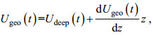 (16)
(16)为了确定Udeep(t)和
其中, 

实际实验的模型中, 设置了实验方案11-1和方案11-2, 方案11-1是时间变化的风应力拖曳系数, 方案11-2是恒定的风应力拖曳系数。实际实验的参数设置如下:风应力拖曳系数初始猜想值设为0.0012;根据Santiago-Mandujano等(1990)和Hui等(2016), 垂向涡动粘性系数设为:

其中, Az是垂向涡粘系数, u10和v10分别是海表面上方10m水平方向的风速分量; 以30min的时间间隔和1m的深度间隔积分10d;初始状态使用BTM站点2005年12月21日0时线性插值后的流速观测值, 风速时间序列使用计算出的U10估计值, 将12月21日0时—12月22日0时作为冷启动的时间; 其余参数的设置与理想实验相同。
实际实验中, 在海面下20.69、26.69、50.69和74.69m处的模拟流速和观测流速u和v的时间序列对比见图 11; 方案11-1和方案11-2大致再现了74.69m以上的观测流速, 模拟流速的相位和振幅与观测流速具有良好的一致性, 不一致的部分有可能是由于其他动力学过程和观测误差叠加到惯性振荡上。在26.69m以上方案11-1比方案11-2反演效果更优, 说明时间变化的风应力拖曳系数的反演对上层流速数据更敏感, 该结论与理想实验相同。方案11-1随迭代步数变化的代价函数如图 12a所示, 代价函数下降了2个数量级; 方案11-1风应力拖曳系数时间序列如图 12b所示, 与图 8a相比, 风应力拖曳系数时间序列变化趋势与U10时间变化趋势具有一定的相似性, 风应力拖曳系数在12月24日和12月27日附近出现两处高峰, 该现象符合物理海洋学现有认知, 即风应力拖曳系数与风速之间成正相关性。方案11-1中2005年12月22日10:30的模拟流速和观测流速的Ekman螺旋对比如图 13所示, 可以看到两者之间具有较好的一致性, 表明通过优化时间变化的风应力系数, 流速的模拟结果能够重现观测数据的基本特征; 同时可以看到, 两者之间有一定的偏差, 这可能是由于模型本身的缺陷和观测数据的误差所致, 使模拟结果不能完全重现观测数据的信息。
 |
| 图 11 方案11-1和方案11-2中20.69, 26.69, 50.69和74.69m处观测和模拟的Ekman东向流速Uek时间序列(a、c、e)以及北向流速Vek时间序列(b、d、f) Fig. 11 The time series of observed and modelled Ekman eastward current velocity (a, c, e) and northward current velocity (b, d, f) at 20.69 m, 26.69 m, 50.69 m and 74.69 m in Cases 11-1 and Cases 11-2, respectively |
 |
| 图 12 方案11-1的log(J/J0)随迭代步数的变化(a)和WSDC反演值时间序列(b) Fig. 12 The values of log(J/J0) vs the iterations (a) and the time series of WSDC (b) inverted in Case 11-1 |
 |
| 图 13 方案11-1在23.69、29.69、35.69、41.69、47.69、53.69和59.69m处模拟和观测的Ekman螺旋结构 Fig. 13 The modeled and observed Ekman spiral in Cases 11-1 at depth 23.69m, 29.69m, 35.69m, 41.69m, 47.69m, 53.69m, and 59.69m 注:观测时间是2005年12月22日10:30 |
本文采用一个改进的Ekman模型, 基于时间分布参数设置的假设, 建立相关算法, 利用伴随同化方法反演了随时间变化的风应力拖曳系数, 主要运行了孪生实验和实际实验。在孪生实验中, 共设置了10组实验, 包括风速分布、风应力系数分布、风应力系数初始猜测值、独立风应力系数个数、观测数据误差和观测深度。第1—6组实验, 验证了不同风速分布下均能成功反演出不同风应力拖曳系数分布。第7组实验测试了5种不同的风应力系数初始猜测值, 初始猜测值越接近给定的初始值, 反演结果越好。第8组实验表明独立风应力拖曳系数个数和位置的选取会显著影响反演结果, 选取合理有利于提高反演效率及减少观测数据误差。第9组实验探讨了模型对观测数据误差的容忍度, 观测数据误差在10%以下能取得有效反演结果。第10组实验比较了使用不同观测层位的影响, 表明反演结果对观测数据的表层和次表层流速更为敏感。这部分的工作分析了变分最优控制方法反演时间变化风应力拖曳系数的主要敏感性因素, 证明了该方法的可行性, 然后尝试了实际实验的探索。
在实际实验中, 利用百慕大锚系实验平台的风速和流速数据, 风速数据利用Large等(1995)提出的公式和Zedler(1999)概述的方法计算出U10, 流速数据利用Zhang等(2009)和Roach等(2015)提出的方法除去周期性潮流和地转流成分后得到Ekman流。反演出的流速成功再现了74.69m以上的观测流速, 并确定2005年12月22日0点—2005年12月29日0点时间段内该区域随时间变化的风应力拖曳系数最优分布。
我们的工作进一步证实了伴随同化方法确定最优参数的能力, 并提供了一种有效的方法来确定时间变化的风应力拖曳系数分布。在实施该方法的过程中, 初始条件、时间长度、边界条件等的输入, 乃至风场驱动的变化, 都会影响参数分布的最优估计, 所以在实际观测的探讨中要具体地点和时间具体分析, 才能得到所研究区域的时间变化风应力拖曳系数的最优估计。未来将进行大风速(最大风速大于35m/s)期间风应力系数估计, 尝试反演台风期间的风应力系数时间分布。
吕咸青. 2001. 数据同化反演风应力拖曳系数以及垂向涡动黏性系数的分布. 海洋学报, 23(1): 13-20 DOI:10.3321/j.issn:0253-4193.2001.01.002 |
Black W J, Dickey T D, 2008. Observations and analyses of upper ocean responses to tropical storms and hurricanes in the vicinity of Bermuda. Journal of Geophysical Research:Oceans, 113(C8): C08009 |
Chereskin T K, 1995. Direct evidence for an Ekman balance in the California Current. Journal of Geophysical Research:Oceans, 100(C9): 18261-18269 DOI:10.1029/95JC02182 |
Daley R, 1991. Atmospheric data analysis. Cambridge, UK: Cambridge University Press
|
Das S K, Lardner R W, 1991. On the estimation of parameters of hydraulic models by assimilation of periodic tidal data. Journal of Geophysical Research:Oceans, 96(C8): 15187-15196 DOI:10.1029/91JC01318 |
Das S K, Lardner R W, 1992. Variational parameter estimation for a two-dimensional numerical tidal model. International Journal for Numerical Methods in Fluids, 15(3): 313-327 DOI:10.1002/fld.1650150305 |
Dickey T, Frye D, McNeil J et al, 1998. Upper-ocean temperature response to hurricane felix as measured by the Bermuda Testbed Mooring. Monthly Weather Review, 126(5): 1195-1201 DOI:10.1175/1520-0493(1998)126<1195:UOTRTH>2.0.CO;2 |
Dickey T, Zedler S, Yu X et al, 2001. Physical and biogeochemical variability from hours to years at the Bermuda Testbed Mooring site:June 1994-March 1998. Deep Sea Research Part Ⅱ:Topical Studies in Oceanography, 48(8-9): 2105-2140 DOI:10.1016/S0967-0645(00)00173-9 |
Edson J B, Jampana V, Weller R A et al, 2013. On the exchange of momentum over the open Ocean. Journal of Physical Oceanography, 43(8): 1589-1610 DOI:10.1175/JPO-D-12-0173.1 |
Evensen G, 1992. Using the extended Kalman filter with a multilayer quasi-geostrophic ocean model. Journal of Geophysical Research:Oceans, 97(C11): 17905-17924 DOI:10.1029/92JC01972 |
Evensen G, Van Leeuwen P J, 1996. Assimilation of Geosat altimeter data for the Agulhas current using the ensemble Kalman filter with a quasigeostrophic model. Monthly Weather Review, 124(1): 85-96 DOI:10.1175/1520-0493(1996)124<0085:AOGADF>2.0.CO;2 |
Ferreira V G, Mangiavacchi N, Tomé M F et al, 2004. Numerical simulation of turbulent free surface flow with two-equation k-ε eddy-viscosity models. International Journal for Numerical Methods in Fluids, 44(4): 347-375 DOI:10.1002/fld.641 |
Fisher M, Courtier P, 1995. Estimating the covariance matrices of analysis and forecast errors in variational data assimilation. ECMWF Technical Memorandum, 22
|
Garratt J R, 1977. Review of drag coefficients over oceans and continents. Monthly Weather Review, 105(7): 915-929 DOI:10.1175/1520-0493(1977)105<0915:RODCOO>2.0.CO;2 |
Gharamti M E, Tjiputra J, Bethke I et al, 2017. Ensemble data assimilation for ocean biogeochemical state and parameter estimation at different sites. Ocean Modelling, 112: 65-89 DOI:10.1016/j.ocemod.2017.02.006 |
Gill P E, Murray W, Wright M H, 1981. Practical Optimization. Mathematical Gazette, pas-104(2): 180
|
Heemink A W, Mouthaan E E A, Roest M R T et al, 2002. Inverse 3D shallow water flow modelling of the continental shelf. Continental Shelf Research, 22(3): 465-484 DOI:10.1016/S0278-4343(01)00071-1 |
Hui Z L, Xu Y S, 2016. The impact of wave-induced Coriolis-Stokes forcing on satellite-derived ocean surface currents. Journal of Geophysical Research:Oceans, 121(1): 410-426 DOI:10.1002/2015JC011082 |
Hwang P A, 2005. Temporal and spatial variation of the drag coefficient of a developing sea under steady wind-forcing. Journal of Geophysical Research:Oceans, 110(C7): C07024 |
Jarosz E, Mitchell D A, Wang D W et al, 2007. Bottom-up determination of Air-Sea momentum exchange under a major tropical cyclone. Science, 315(5819): 1707-1709 DOI:10.1126/science.1136466 |
Jiang S N, Dickey T D, Steinberg D K et al, 2007. Temporal variability of zooplankton biomass from ADCP backscatter time series data at the Bermuda Testbed Mooring site. Deep Sea Research Part Ⅰ:Oceanographic Research Papers, 54(4): 608-636 DOI:10.1016/j.dsr.2006.12.011 |
Jones J E, Davies A M, 1998. Storm surge computations for the Irish Sea using a three-dimensional numerical model including wave-current interaction. Continental Shelf Research, 18(2-4): 201-251 DOI:10.1016/S0278-4343(97)00062-9 |
Kalman R E, 1960. A New Approach to Linear Filtering and Prediction Problems. Journal of Basic Engineering, 82(1): 35-45 DOI:10.1115/1.3662552 |
Kim H J, Ahn J B, 2015. Improvement in prediction of the arctic oscillation with a realistic ocean initial condition in a CGCM. Journal of Climate, 28(22): 8951-8967 DOI:10.1175/JCLI-D-14-00457.1 |
Kirincich A R, Barth J A, 2009. Time-varying across-shelf Ekman transport and vertical eddy viscosity on the inner shelf. Journal of Physical Oceanography, 39(3): 602-620 DOI:10.1175/2008JPO3969.1 |
Konishi T, Kinosita T, Takahashi H, 1985. Storm surges in estuaries: the 17th Joint Meeting US Japan Panel on Wind and Seismic Effects, Tsukuba Japan. Japan: UJNR, 735-749
|
Large W G, Pond S, 1981. Open ocean momentum flux measurements in moderate to strong winds. Journal of Physical Oceanography, 11(3): 324-336 DOI:10.1175/1520-0485(1981)011<0324:OOMFMI>2.0.CO;2 |
Large W G, Crawford G B, 1995. Observations and simulations of upper-ocean response to wind events during the ocean storms experiment. Journal of Physical Oceanography, 25(11): 2831-2852 DOI:10.1175/1520-0485(1995)025<2831:OASOUO>2.0.CO;2 |
Large W G, Yeager S G, 2009. The global climatology of an interannually varying air-sea flux data set. Climate Dynamics, 33(2-3): 341-364 DOI:10.1007/s00382-008-0441-3 |
Lenn Y D, Chereskin T K, 2009. Observations of Ekman currents in the Southern Ocean. Journal of Physical Oceanography, 39(3): 768-779 DOI:10.1175/2008JPO3943.1 |
Leredde Y, Devenon J L, Dekeyser I, 1999. Turbulent viscosity optimized by data assimilation. Annales Geophysicae, 17(11): 1463-1477 DOI:10.1007/s00585-999-1463-9 |
Liu J, Dai J J, Xu D F et al, 2018. Seasonal and interannual variability in coastal circulations in the northern South China Sea. Water, 10(4): 520 DOI:10.3390/w10040520 |
Luenberger D G, Ye Y Y, 1984. Linear and nonlinear programming. New York, NY: Springer, 105-110
|
Lv X Q, Wu Z K, Gu Y et al, 2004. Study on the adjoint method in data assimilation and the related problems. Applied Mathematics and Mechanics, 25(6): 636-646 DOI:10.1007/BF02438206 |
Maurer K D, Bohrer G, Ivanov V Y, 2015. Large eddy simulations of surface roughness parameter sensitivity to canopy-structure characteristics. Biogeosciences, 11(11): 16349-16389 |
Mellor G L, 2004. User's guide for a three-dimensional, primitive equation, numerical ocean model. Princeton, USA:Princeton University, 56
|
Navon I M, 1998. Practical and theoretical aspects of adjoint parameter estimation and identifiability in meteorology and oceanography. Dynamics of Atmospheres and Oceans, 27(1-4): 55-79 DOI:10.1016/S0377-0265(97)00032-8 |
O'Brien, 1986. Advanced physical oceanographic numerical modelling. Dordrecht: Springer, 127-144
|
Pacanowski R C, Philander S G H, 1981. Parameterization of vertical mixing in numerical models of tropical oceans. Journal of Physical Oceanography, 11(11): 1443-1451 DOI:10.1175/1520-0485(1981)011<1443:POVMIN>2.0.CO;2 |
Peng S Q, Li Y N, 2015. A parabolic model of drag coefficient for storm surge simulation in the South China Sea. Scientific Reports, 5: 15496 DOI:10.1038/srep15496 |
Phillips H E, Bindoff N L, 2015. On the nonequivalent barotropic structure of the Antarctic Circumpolar Current:An observational perspective. Journal of Geophysical Research:Oceans, 119(8): 5221-5243 |
Polton J A, Lenn Y D, Elipot S et al, 2013. Can drake passage observations match Ekman's classic theory. Journal of Physical Oceanography, 43(8): 1733-1740 DOI:10.1175/JPO-D-13-034.1 |
Powell M D, Vickery P J, Reinhold T A, 2003. Reduced drag coefficient for high wind speeds in tropical cyclones. Nature, 422(6929): 279-283 DOI:10.1038/nature01481 |
Ralph E A, Niiler P P, 1999. Wind-driven currents in the tropical pacific. Journal of Physical Oceanography, 29(9): 2121-2129 DOI:10.1175/1520-0485(1999)029<2121:WDCITT>2.0.CO;2 |
Roach C J, Phillips H E, Bindoff N L et al, 2015. Detecting and characterizing Ekman currents in the southern Ocean. Journal of Physical Oceanography, 45(5): 1205-1223 DOI:10.1175/JPO-D-14-0115.1 |
Santiago-Mandujano F, Firing E, 1990. Mixed-layer shear generated by wind stress in the central equatorial pacific. Journal of Physical Oceanography, 20(10): 1576-1582 DOI:10.1175/1520-0485(1990)020<1576:MLSGBW>2.0.CO;2 |
Sasaki Y, 1970. Some basic formalisms in numerical variational analysis. Monthly Weather Review, 98(12): 875-883 DOI:10.1175/1520-0493(1970)098<0875:SBFINV>2.3.CO;2 |
Thacker W C, Long R B, 1988. Fitting dynamics to data. Journal of Geophysical Research:Atmospheres, 93(C2): 1227-1240 DOI:10.1029/JC093iC02p01227 |
Ullman D S, Wilson R E, 1998. Model parameter estimation from data assimilation modeling:Temporal and spatial variability of the bottom drag coefficient. Journal of Geophysical Research:Oceans, 103(C3): 5531-5549 DOI:10.1029/97JC03178 |
Wakelin S L, Holt J T, Proctor R, 2009. The influence of initial conditions and open boundary conditions on shelf circulation in a 3D ocean-shelf model of the North East Atlantic. Ocean Dynamics, 59(1): 67-81 DOI:10.1007/s10236-008-0164-3 |
Wang Y G, Qiao F L, Fang G H et al, 2010. Application of wave-induced vertical mixing to the K profile parameterization scheme. Journal of Geophysical Research:Oceans, 115(C9): C09014 |
Weller R A, Plueddemann A J, 1996. Observations of the vertical structure of the oceanic boundary layer. Journal of Geophysical Research:Oceans, 101(C4): 8789-8806 DOI:10.1029/96JC00206 |
Wu J, 1980. Wind-stress coefficients over sea surface near neutral conditions-A revisit. Journal of Physical Oceanography, 10(5): 727-740 DOI:10.1175/1520-0485(1980)010<0727:WSCOSS>2.0.CO;2 |
Wu J, 1982. Wind-stress coefficients over sea surface from breeze to hurricane. Journal of Geophysical Research:Oceans, 87(C12): 9704-9706 DOI:10.1029/JC087iC12p09704 |
Yoshikawa Y, Endoh T, Matsuno T et al, 2010. Turbulent bottom Ekman boundary layer measured over a continental shelf. Geophysical Research Letters, 37(15): L15605 |
Yu L S, O'Brien J J, 1991. Variational estimation of the wind stress drag coefficient and the oceanic eddy viscosity profile. Journal of Physical Oceanography, 21(5): 709-719 DOI:10.1175/1520-0485(1991)021<0709:VEOTWS>2.0.CO;2 |
Yu L S, O'Brien J J, 1992. On the Initial condition in parameter estimation. Journal of Physical Oceanography, 22(11): 1361-1364 DOI:10.1175/1520-0485(1992)022<1361:OTICIP>2.0.CO;2 |
Zedler S E, 1999. Observations and modeling of the ocean's response to Hurricane Felix at the Bermuda Testbed Mooring. Santa Barbara, USA: University of California
|
Zedler S E, Dickey T D, Doney S C et al, 2002. Analyses and simulations of the upper ocean's response to hurricane Felix at the Bermuda Testbed Mooring site:13-23 August 1995. Journal of Geophysical Research:Oceans, 107(C12): 25-1 |
Zhang J C, Lu X Q, 2008. Parameter estimation for a three-dimensional numerical barotropic tidal model with adjoint method. International Journal for Numerical Methods in Fluids, 57(1): 47-92 DOI:10.1002/fld.1620 |
Zhang Q L, Gao Y Q, Lv X Q, 2015. Estimation of oceanic eddy viscosity profile and wind stress drag coefficient using adjoint method. Mathematical Problems in Engineering, 2015: 309525
|
Zhang Y W, Tian J W, Xie L L, 2009. Estimation of eddy viscosity on the South China Sea shelf with adjoint assimilation method. Acta Oceanologica Sinica, 28(5): 9-16 |
Zijlema M, Van Vledder G P, Holthuijsen L H, 2012. Bottom friction and wind drag for wave models. Coastal Engineering, 65: 19-26 DOI:10.1016/j.coastaleng.2012.03.002 |